Differential & integral models

From changing states to fields and integral operators.

Numerical ODEs, two-point BVPs, scalar PDEs, eigenvalues and second-kind integral equations—with documented mathematical assumptions and limits.

Ordinary differential equations and trajectories.

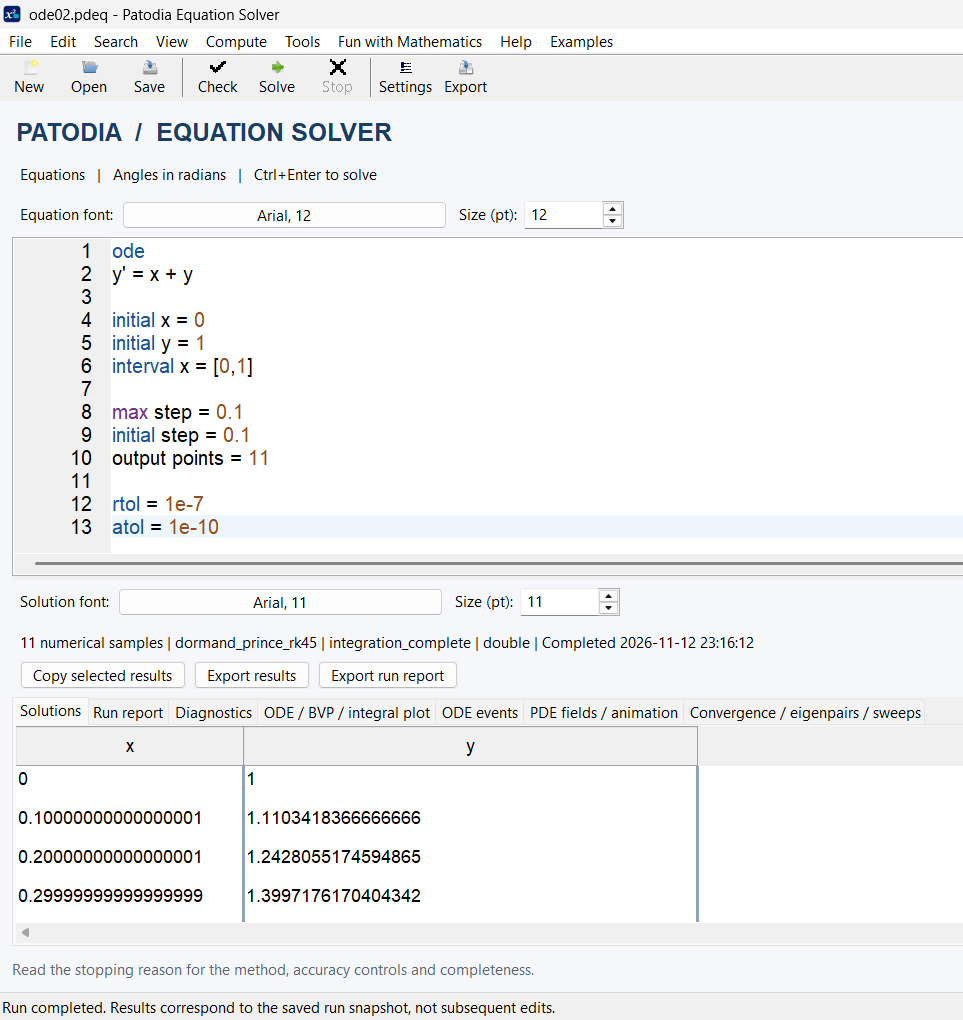
Enter a scalar or coupled initial-value ODE with its initial conditions and integration interval. Supported fixed-step and adaptive methods include RK4 and RK45, with other methods for appropriate problems. Configure output sampling so the observation times of interest actually occur in the reported table.

ode
y' = -y
initial t = 0
initial y = 1
interval t = [0,1]
method = RK45
output step = 0.05

Reference: y(t)=exp(−t), hence y(1)=e⁻¹. State values and errors depend on tolerance and sampling.

ODE numerical trajectory output in Version 4.0 — Ordinary differential equations · Actual Version 4.0 application screenshot; select to enlarge

Boundary-value problems

Two-point boundary problems specify conditions at different places, rather than all conditions at one initial point. The BVP service supports documented regular problems, endpoint conditions and method controls. Nonlinear solutions may depend on a starting curve and should not be assumed to enumerate every solution branch.

bvp
y'' = -2
interval x = [0,1]
boundary left y = 0
boundary right y = 0
output step = 0.1

The exact benchmark is y(x)=x(1−x), giving y(0.5)=0.25. Compare solver values with their actual reported grid coordinates.

PDE fields: Laplace, Poisson, heat and wave.

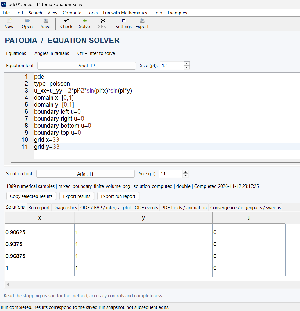
Supported scalar PDEs include Laplace/Poisson on rectangular domains and one-dimensional heat and wave formulations with documented boundary types. Grid resolution and time-step constraints affect accuracy and stability. General nonlinear PDEs on arbitrary geometries are not implied.

pde
type = poisson
u_xx + u_yy = -2*pi^2*sin(pi*x)*sin(pi*y)
domain x = [0,1]
domain y = [0,1]
boundary left u = 0
boundary right u = 0
boundary bottom u = 0
boundary top u = 0
grid x = 33
grid y = 33

Manufactured reference: u(x,y)=sin(πx)sin(πy); the exact centre value is 1. A discrete grid approximation may differ.

Poisson PDE output shown in Version 4.0 — Poisson equation results · Actual Version 4.0 application screenshot; select to enlarge

Fredholm and Volterra integral equations.

The integral service solves supported linear integral equations of the second kind using specified forcing, kernel, interval, lambda and grid. Fredholm and Volterra types differ in the integration range and discretization. General nonlinear, first-kind or arbitrary singular kernels are outside the documented mode.

integral
type = volterra
interval x = [0,1]
forcing = 1
kernel = 1
lambda = 1
grid x = 65
exact solution = exp(x)

This benchmark has exact solution y(x)=exp(x); the numerical result can be compared with that function on the output grid.

Volterra or Fredholm integral equation output from Version 4.0 — Integral equations · Actual Version 4.0 application screenshot; select to enlarge

Eigenvalue problems and quality controls

The eigen service supports documented Sturm–Liouville-type formulations, allowing users to calculate selected eigenpairs and mode shapes. Eigenvalue accuracy depends on mesh discretization, scaling and boundary formulation.

For all services, differentiate the mathematical reference solution from a discrete numerical approximation. Inspect the actual solver status, accepted flags, convergence information and residuals; independently verify any safety-critical or publishable result.

Consult the complete syntax and numerical-method guidance

The User Guide 4.0 PDF is available to read or download. Browse all six documents on the Resources page.

Open / Download PDF ↗