FOR SOFTWARE VENDORS & PRODUCT TEAMS

Build more capability
into your software.
Embed the mathematics.

Multiple real-solution discovery and practical heuristic optimization for engineering, planning and scientific software. Seek useful, verified candidates within the computational effort available for your decision.

Discuss an OEM evaluation Try Optimizer Try Equation Solver

Patodia Optimizer & Equation Solver
Native C++ engines · Callable library interfaces · Company-specific OEM agreements

2 complementary enginesOptimization + equation solving

100% known-root coverageAll 20 test cases, both precision modes, at 2 s and 5 s

Up to 18,512 citiesIn the supplied TSP benchmark

PRACTICAL NUMERICAL SEARCH

Useful answers.
Controllable search effort.

A feasible decision can be useful before global optimality is established. Our heuristic search prioritizes finding and improving numerical candidates, with acceptance checks against the represented model and configured tolerances.

Use the time available for the actual decision: explore alternative equation solutions, improve an operating plan, or continue a supported saved optimization search when more computation becomes available. Evaluate feasibility and objective quality separately from mathematical proof.

Set the allowance

Configure cooperative time budgets, seeds and applicable iteration or node limits. Inspect the stopping reason and the best accepted result.

Bound the work

Supported scalar NLP/MINLP work mode offers deterministic work units. A fixed work budget is distinct from a wall-clock deadline.

Preserve progress

Save a compatible work-mode checkpoint and resume with additional work, retaining the best verified incumbent instead of starting the supported search again.

Time allowances are cooperative, not hard real-time deadlines. Setup, indivisible numerical operations, verification and result or checkpoint output can add latency. Work-mode and ordinary timed search use different search policies; neither is a universal objective-quality replacement for the other.

THE PRODUCT FAMILY

One partnership.
Two numerical capabilities.

Choose the engine that fits your workflow, or evaluate both. Retain your product experience while adding the numerical component behind it.

01 OBJECTIVE-DRIVEN SEARCH

Patodia Optimizer

Improve decisions while respecting the model’s requirements.

Try Optimizer

Mathematical optimization

Linear, mixed-integer linear, nonlinear and mixed-integer nonlinear models. Minimize or maximize an objective subject to represented bounds and constraints.

Operational models

Dedicated services for TSP and vehicle routing, cutting stock, packing, scheduling, rostering, assignment, transportation and resource placement.

Controlled heuristic search

Seek useful feasible candidates within cooperative time allowances and mode-specific work limits. Inspect objectives, stopping reasons and applicable bounds or gaps.

Save and continue

Supported scalar NLP/MINLP work-mode searches can checkpoint and resume with additional work while retaining the best verified incumbent. Requires compatible models, builds and settings.

Model interoperability

Supported LP, MPS and NL imports, native text models and documented modelling workflows. Extended precision is available in supported builds and modes.

Windows executable & DLL; Linux x86-64 executable & .so shared library available.
Linux build targets the CentOS 8 glibc 2.28 baseline.

02 OBJECTIVE-FREE SOLVING

Patodia Equation Solver

Explore alternative real solutions in a single run.

Multiple real solutions

Search for distinct approximate real roots of linear, polynomial and supported transcendental systems, without a user-supplied initial estimate.

Constrained feasibility

Continuous, integer and mixed-integer variables; variable bounds and inclusive inequalities. Automatic range exploration or explicit physical bounds.

Extended precision

Binary128 refinement offers 113 significand bits, approximately 33 significant decimal digits. Residual tolerance is configurable; it does not imply equivalent coordinate accuracy.

Visible discovery times

Per-root acceptance time and time to the last distinct accepted root, together with residuals and stopping status. Separate discovery time from total search time.

Windows executable & DLL; Linux x86-64 executable & .so available.
Linux build targets the CentOS 8 glibc 2.28 baseline.

Model the relationships you need.

Arithmetic, powers, implicit multiplication and scientific notation; supported functions include sin, cos, tan, log, exp, sqrt, abs, atan2, min, max, log1p and expm1. Valid real domains apply; expression support varies by solving and verification mode.

An application built around the native engine

Your equations. A live interface.
Multiple numerical solutions.

See Patodia Equation Solver behind a working web interface. Enter a supported equation system, set the search controls and inspect the returned roots, residuals and discovery times — an example of the engine capability you can evaluate for your own application.

11Coupled equations / unknowns

9Returned solution vectors

1 sConfigured search allowance

< 1e-9Every displayed maximum residual

Web Equation Solver with eleven nonlinear equations, one-second search budget, 1e-9 tolerance and 128-bit precision unchecked — **The model:** eleven coupled equations in x1–x11, using sin, cos, tan, exp and ln, polynomial terms and products between unknowns. The visible settings specify a **one-second allowance**, **1e-9 residual tolerance**, 12,000 starting points, up to 100 solutions and 300 iterations per start. The binary128 option is unchecked.

Web solver reporting nine distinct approximate real solutions, 1.11-second web process elapsed time, 1.00009-second solver runtime and 0.863942605-second last-root acceptance time — **The result:** this web run returned **nine distinct approximate real solution vectors**. The run summary distinguishes **solver runtime: 1.00009 s**, **web-process elapsed time: 1.11 s** and **last distinct root accepted: 0.863942605 s**. The first table view shows the solution indices and initial variable columns.

Continuation of the nine-solution table showing remaining variables, maximum residuals and per-root acceptance times — **The numerical evidence:** the continuation shows the remaining coordinates together with a maximum absolute residual and acceptance time for each solution. The visible residuals are below the configured **1e-9** tolerance. The results summary reports nine accepted solutions; the ninth row is partially below the screenshot viewport. Together, the two table views show all eleven variable columns; the ninth row is partially below the visible table viewport. These are solver-reported checks, not an independent residual recomputation.

A practical example of embedding.

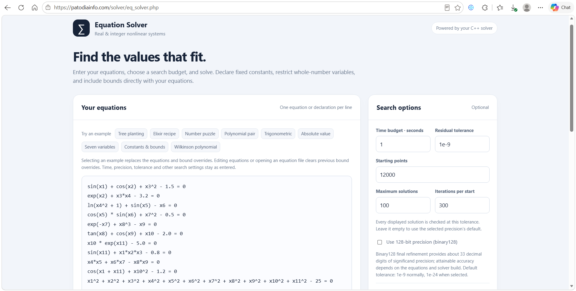
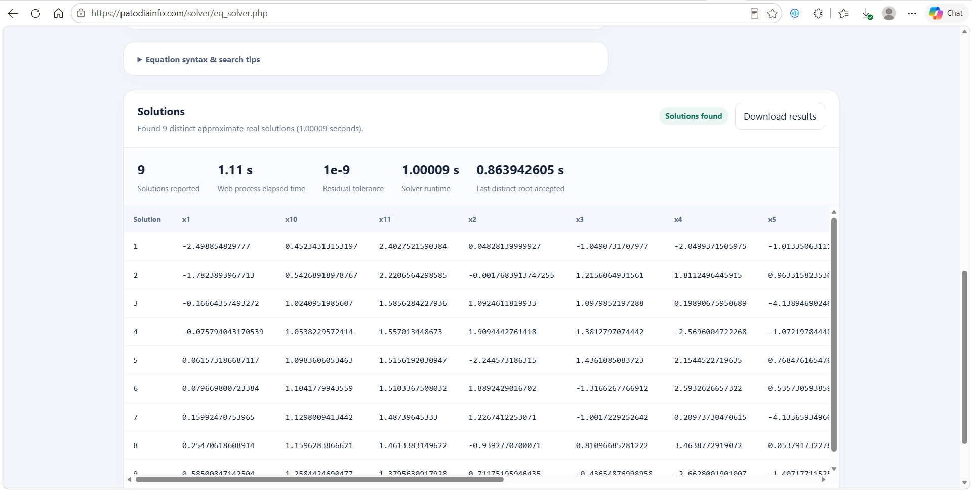
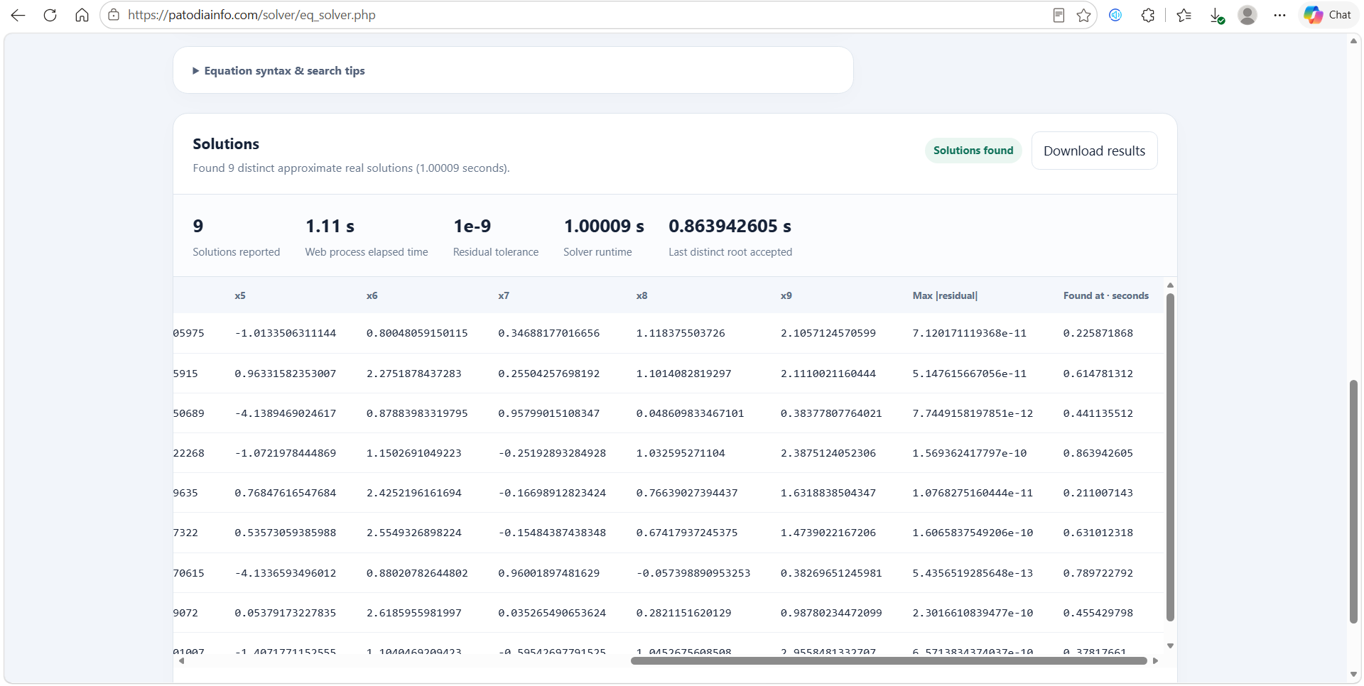
The web page provides the model editor, search controls and results presentation. The native C++ engine supplies numerical search and diagnostics. Evaluate the matching executable or library interface behind your own engineering, scientific or planning software.

Bring a representative model.

Open the live Equation Solver page, enter supported equations, constants and variable declarations, and try bounds or inclusive inequalities where appropriate. Review the results against your application's numerical requirements.

Try your own equations ↗Discuss embedding in your application →Explore the Excel add-in →

Screenshots supplied by Patodia Infotech from one web run. The one-second setting is a cooperative search allowance; measured solver runtime and web-process elapsed time are reported separately. The 1.11-second figure is the application's web-process measurement, not a measured browser round trip. This run was not independently reproduced for this page; hardware and executable hashes are not provided. General search is heuristic and does not establish root completeness or guarantee the same results on another run or model.

WHERE TO START

A numerical component for your domain.

Process & formulation software

Steady-state balances, equilibrium relationships, alternative operating points and constrained operating decisions.

Robotics & engineering tools

Nonlinear geometric relationships, alternative mechanism configurations and parameter-fitting models.

Planning & logistics applications

Routing, allocation, packing and scheduling through dedicated supported model services.

These are evaluation starting points. Suitability and scale are established using your representative models and requirements.

MEASURED RESULTS

Evidence you can inspect.
Problems you can bring.

Our supplied benchmark reports provide a starting point. The next step is a reproducible evaluation against your own models and acceptance criteria.

EQUATION SOLVER

Every known root matched at 2 s and 5 s.

40 / 40 runs at each budget: all 20 bounded test cases in both normal and extended precision.

20 bounded cases × 3 time budgets × 2 precision modes; seed 42.

Budget	Complete runs	Matched / expected*
1 s	39 / 40	1,027 / 1,028
2 s	40 / 40	1,028 / 1,028
5 s	40 / 40	1,028 / 1,028

*Root occurrences summed across cases and precision modes. The only partial run matched 255 of 256 roots at 1 second in extended mode; both longer budgets matched 256.

Normal tolerance 1e-9; extended tolerance 1e-24. Includes structured sign-combination tests as well as polynomial, transcendental, nonsmooth and mixed-integer examples.

DISCOVERY TIMING

See when the results arrive.

For the eight-variable, 256-root extended-mode test with a 2-second allowance:

Last accepted root: 1.010291 s
Total solver time: 2.0002 s
Harness wall time: ≈ 2.1198 s

Root timings show acceptance within the run. They are distinct from application latency and do not establish completeness.

OPTIMIZER / PROCESS ENGINEERING

Process-engineering nonlinear and MINLP benchmarks.

Seven MINLPLib process-profile instances. Five seeds (38–42). Three allowances (5, 15 and 30 seconds), per precision mode.

210 recorded runs

105 normal + 105 extended

100 / 105 accepted

Normal-precision report

95 / 105 accepted

Extended-precision report

Best accepted normal-precision candidates are shown below. All seven models are minimization problems. Six best results differ from their listed primal references by less than 0.000001%; General heat exchange retains a substantial gap.

Model	Best objective	Primal reference	Reference difference*	Allowance / seed
alkyl	-1.7649996476604	-1.76499965	< 0.000001%	5 s / 38
process	-1161.336602411	-1161.336602	< 0.000001%	5 s / 40
haverly	-400.00000001404	-400	< 0.000001%	30 s / 40
pooling_haverly1pq	-400.00000000793	-400	< 0.000001%	5 s / 38
pooling_haverly2pq	-600.0000000072	-600	< 0.000001%	5 s / 38
heatexch_gen1	229590.92988541	154895.933	48.2227%	30 s / 38
heatexch_spec1	154997.33486584	154997.3349	< 0.000001%	30 s / 38

*Magnitude of 100 × (objective − reference) / max(1, |reference|), calculated from the report values. Tiny differences on either side of a rounded reference do not prove a better optimum. These are comparisons with listed primal references, not certified optimality gaps. Best results across configurations are not averages or guaranteed repeatable outcomes.

Repeated-run quality, extended precision and benchmark conditions

General heat exchange: at the 30-second allowance, normal precision accepted 5 / 5 runs, with median objective 391,713.90639932 and best objective 229,590.92988541. The best result is therefore substantially better than the median; both remain above the 154,895.933 reference. This report records the best PHP-harness result, not an independently reproduced direct-CLI guarantee.

Specialized heat exchange: normal precision accepted 0 / 5 runs at 5 seconds, 5 / 5 at 15 seconds and 5 / 5 at 30 seconds. At 30 seconds, its median objective was 154,997.33486584, essentially matching the listed reference to its reported precision.

Extended precision is a numerical option, not an objective-quality promise. In the separate extended report, the best General objective was 600,766.86660394 (287.8519% reference difference), and the best Specialized objective was 272,480.35426541 (75.7968%). Specialized accepted no candidate in the ten runs at the two shorter allowances, then accepted 5 / 5 at 30 seconds. More arithmetic precision did not yield a better optimization result in these heat-exchanger tests.

Sources: supplied process-profile reports dated 16 October 2026; normal report generated 14:11:02 UTC and extended report generated 09:36:58 UTC. These are separate report snapshots, not a controlled same-build precision comparison. Acceptance and violations are solver-reported; the runner does not independently certify feasibility. Exact executable hashes, hardware and complete tolerance settings must be retained in an OEM reproduction. No competing solver was benchmarked. The process profile includes continuous nonlinear as well as mixed-integer nonlinear formulations; 210 runs does not mean 210 distinct MINLP models.

Configured allowances are not measured application latency. For example, normal Specialized at the 30-second allowance had median harness wall time 30.1102 seconds. These historical observations do not establish an absolute deadline or performance on another machine, build or model.

OPTIMIZER / TSP

Tour quality across eight problem sizes.

23 usable run results. Best observed result per model is shown below.

Model	Cities	Listed optimum	Obtained cost	Reference gap	Budget
att48	48	10,628	10,628	0.000%	5 s
bier127	127	118,282	118,282	0.000%	20 s
d493	493	35,002	35,069	0.191%	20 s
dsj1000	1,000	18,660,188	18,791,775	0.705%	60 s
d1655	1,655	62,128	62,712	0.940%	90 s
brd14051	14,051	469,385	478,314	1.902%	180 s
d15112	15,112	1,573,084	1,603,368	1.925%	180 s
d18512	18,512	645,238	658,945	2.124%	180 s

Gap = 100 × (obtained cost − listed optimum) / listed optimum. Best results across tested budgets, not averages. Matching reference costs does not independently certify tour optimality.

Benchmark scope and interpretation

Sources: supplied Equation roots benchmark, 15 October 2026; process-profile reports, 16 October 2026; and TSP Benchmark Report, 8 October 2026. Equation and TSP observations use one seed per configuration; process-profile observations use five. No competing solver was run. Reports do not identify CPU/RAM or executable hashes, so these historical observations are not portable latency guarantees or benchmarks of every platform build.

Equation coverage uses known bounded reference roots and printed residual checks; it is not an interval completeness certificate or an independent binary128 residual recomputation. Structured sign-combination tests do not represent arbitrary densely coupled systems. TSP costs do not establish performance on other optimization classes.

Read the capability brief & benchmark details (PDF)

DESIGNED TO BE EMBEDDED

Your interface.
Our numerical engine.

Evaluate the command line first, then integrate using the matching native library interface and language adapter.

Native deployment

Both Optimizer and Equation Solver are available as Windows executables and DLLs, and as Linux x86-64 executables and .so shared libraries. Linux builds target the CentOS 8 glibc 2.28 baseline. Match architecture and runtime dependencies to your application.

Language interoperability

C-compatible interfaces enable calls from C, C++ and other foreign-function environments. The Optimizer Developer Guide includes C, C++, C#, Python, Java, Julia and PHP examples for DLL or shared-library integration. Validate the matching adapter and target runtime as part of evaluation.

Inspectable results

Review residuals, feasible candidates and stopping status. Equation Solver offers JSON results with high-precision values retained as decimal strings, plus individual-root and last-root timings.

Predictable integration starts with explicit controls.

Use supported progress callbacks and cooperative cancellation with the appropriate API. Independent typed-core contexts support concurrent mathematical solves; general legacy calls serialize. Measure total application latency on representative models and use a supervised worker process when the host application needs an external deadline.

Discovery, accuracy and certification are separate.

Native multiple-root search is heuristic. A small residual alone does not prove coordinate accuracy, completeness or global optimality. Optional IBEX-based verification supports a narrower class of continuous square equality systems in a stated finite domain; completeness is reported only when the required coverage and root checks succeed.

TECHNICAL DOCUMENTATION

Read the details before you integrate.

Explore model syntax and search controls in the User Guide, compilation and language integration in the Developer Guide, and the underlying process benchmark records.

LET’S TEST YOUR USE CASE

Bring the problems
your customers need solved.

We propose an OEM evaluation around your software, representative models and measurable goals. Commercial terms reflect the agreed embedding, redistribution, deployment and support scope.

Request an OEM evaluation

Email panna@patodiainfo.com

01
Define the fit
Share model types, sizes, platform and the capability you want to add.
02
Evaluate together
Agree datasets, tolerances, time budgets, repeatability and success criteria.
03
Plan the integration
Review interfaces, dependencies, distribution rights and support needs.